Data Reprocessing Campaign (REPRO1)
Objective
The Analysis Centers (ACs) of the International GNSS Service are in the process of reanalyzing the full history of GPS data collected by the IGS global network since 1994 in a fully consistent way using the latest models and methodology. This is the first such full reprocessing by the IGS, but it is expected to be repeated in the future as further analysis changes are made.
The expected Analysis Center and combined IGS products include:
- daily GPS orbits & satellite clocks
- 15-minute intervals (SP3c format)
- satellite clocks in IGS timescale (loosely aligned to GPS time)
- daily satellite & tracking station clocks
- 5-minute intervals (clock RINEX format)
- in IGS timescale (loosely aligned to GPS time)
- daily Earth rotation parameters (ERPs)
- from SINEX & classic orbit combinations (IGS erp format)
- x & y coordinates of pole
- rate-of-change of x & y pole coordinates
- excess length-of-day (LOD)
- weekly terrestrial coordinate frames with ERPs
- with full variance-covariance matrix (SINEX format)
- possible other products ?
- ionosphere maps, tropospheric zenith path delays, etc
- not part of this first campaign
The participating Analysis Centers contributing complete solutions to this effort are:
- CODE — Center for Orbit Determination in Europe, Switzerland
- EMR — Natural Resources Canada, Canada
- ESA — European Space Operations Centre (ESOC), ESA, Germany
- GFZ — GeoForschungsZentrum/Potsdam, Germany
- JPL — Jet Propulsion Laboratory, USA
- MIT — Massachusetts Institute of Technology, USA
- NGS — National Geodetic Survey, NOAA, USA
- PDR — GeoForschungsZentrum/Potsdam & Technical University of Dresden, Germany
- SIO — Scripps Institution of Oceanography, USA
In addition, some centers provide weekly SINEX solutions to help densify the terrestrial reference frame, particularly for GPS stations located near tide gauges (associated with the TIGA Pilot Project); work is underway to perhaps include associated satellite orbits and clocks:
Summaries of the analysis strategies and procedures for each AC are posted at the IGS Central Bureau. Submitted AC solution files are posted at this GFZ site.
The product combination centers are:
- NRCan — Natural Resources Canada, Canada
- SINEX combination — as of mid-Feb. 2009, results posted for years 2000-2008 (see below)
- NCL — University of Newcastle-upon-Tyne, UK
- SINEX combinations
- GFZ — GeoForschungsZentrum/Potsdam, Germany
- ftp directories for repro1 weekly summary reports & daily product files from orbit combinations
- a summary of all AC submissions is given in the ftp file “Submission_statistics_*.txt” where the * is the date of last update
- NRL — Naval Research Laboratory, USA
- clock & timescale combination results not yet available
Essential elements of the analysis procedures used by all participating centers include:
- try to complete archives for missing or useful data sets
- focus on as many tide gauge stations as possible
- also try to include NGA/NIMA tracking stations
- try to include all GPS stations co-located with other techniques
- use “absolute” antenna calibrations for satellite transmit & ground receive antennas
- background information
- implemented in IGS operational solutions starting GPS week 1400
- current antenna calibration file is igs05.atx in ANTEX format
- use IGS05 reference frame (aligned to ITRF2005)
- background information, including station-specific corrections to account for effect of new antenna calibration model
- implemented in IGS operational solutions starting GPS week 1400
- current reference frame file is IGS05_repro.snx in SINEX format
- currently known or suspected discontinuities in the IGS station positions are tabulated in SINEX format
- IERS Conventions 2003 generally implemented
- with occasional updates posted by the IERS Conventions Center
- updated model for station displacements due to ocean tidal loading
- site-dependent load coefficients recommended using FES2004 ocean tide model
- corrections for counter-balancing center-of-mass motion of the solid Earth should be included in site coefficients
- whole-Earth center-of-mass corrections should also be applied in generating SP3 orbits as described in updated IERS Conventions Chapter 7
- no non-tidal loading displacements should be applied to station positions
- see this position paper on principles for conventional contributions to modeled station displacements, presented at the IERS workshop on Conventions, held at BIPM, 20-21 September 2007
- updated models for tropospheric propagation delays
- refer to revised IERS Conventions Chapter 9
- a priori meteorological data sources:
- [1] local sensor met files (which however are only available for a few sites), or
- [2] barometric pressure values computed using the location- & season-dependent GPT model, or
- [3] retrieved from a numerical weather model, as for the ECMWF global values provided by the service at the Technical University of Vienna in the form of gridded hydrostatic zenith delays (see below)
- the a priori hydrostatic delay in the zenith direction should be computed from the surface pressure according to the formula of Saastamoinen (1972) as given by Davis et al. (1985) and shown as eqn (11) in the revised IERS Conventions Chapter 9
- or retrieved directly in this form based on a numerical weather model, as for the gridded ECMWF values provided by the
service at the Technical University of Vienna - or alternatively one can use an a priori zenith delay consisting of both the hydrostatic and wet components (using surface temperature values from GPT and a standard relative humidity of about 0.5) to ensure tropospheric parameter adjustments that are more nearly zero-mean
- or retrieved directly in this form based on a numerical weather model, as for the gridded ECMWF values provided by the
- line of sight delays should be computed using either
- [1] the location- & season-dependent GMF mapping function model, or
- [2] or a mapping function based on retrieval coefficients from a numerical weather model, as for the ECMWF global values provided by the service at the Technical University of Vienna for the VMF1 mapping function model
- residual tropospheric delays should be parameterized in the GPS data analysis on the assumption that they are predominantly due to the wet component of the troposphere (wet mapping function partials) & azimuthal gradients, as described in IERS Conventions Chapter 9
- no common model for higher-order ionospheric corrections has been agreed yet
- the IGS master SINEX template file, igs.snx, is updated daily based on the history of IGS site logs & should be used to validate AC SINEX file metadata for information on historic and discontinued sites igs_with_former.snx should be used
- P1-C1 satellite code biases
- see site at Astronomical Institute of the University of Bern for general information, bias tables, and receiver types:
- see ESA/ESOC site for latest version (v6.2) of cc2noncc.f routine:
- for information about biases before 02 April 2000 see this message from Stefan Schaer (10 Feb 2009): “Pre-2000” GPS P1-C1 bias values for IGS reprocessing
Test Results
To evaluate analysis and combination procedures, the ACs have provided test solutions for the first quarter of year 2000. Results from those tests are posted here.
Objective
Before proceeding with the full reprocessing campaign, a 3-month test period at the beginning of year 2000 was chosen to evaluate the analysis procedures and performances of the Analysis Centers (ACs), as well as exercise the reprocessing combinations.
Test Sinex Frame Results
The ACs provided test solutions for the first quarter of year 2000 (GPS weeks 1042-1059; the ESA solutions cover the 14 weeks from 1042-1055). Statistics for the station position residuals (average weighted mean & average standard deviation) from the combination of the weekly SINEX files from each AC, after removing separate Helmert transformations (see following), are tabulated below.
| SINEX Terrestrial Frame Residuals | ||||||||||
| AC code |
# wks |
# sta |
w.r.t. Weekly Combination | w.r.t. Cumulative Combination | ||||||
| N | E | U | N | E | U | |||||
| (mm) | (mm) | (mm) | (mm) | (mm) | (mm) | |||||
| ESA (old) ± |
14 | 107.3 | 0.7 3.3 |
0.2 5.0 |
-2.2 9.5 |
1.0 3.5 |
0.4 5.2 |
-2.2 10.3 |
||
| ESA (new) ± |
14 | 120.5 | 0.6 2.3 |
0.1 3.7 |
-1.0 7.2 |
1.1 2.6 |
0.1 3.9 |
-0.9 8.3 |
||
| MIT ± |
18 | 261.3 | -0.4 1.6 |
-0.1 1.9 |
0.3 5.0 |
0.1 4.5 |
0.1 1.9 |
0.4 5.9 |
||
| NGS (old) ± |
13 | 168.9 | 0.3 3.9 |
0.6 4.8 |
0.6 7.7 |
0.7 4.2 |
0.8 5.1 |
0.7 8.3 |
||
| NGS (new) ± |
18 | 170.1 | -0.4 2.4 |
0.3 2.6 |
-0.7 5.2 |
-0.1 2.7 |
0.4 3.1 |
-0.7 6.3 |
||
| PDR ± |
18 | 151.5 | 0.0 2.0 |
0.2 2.0 |
-0.5 5.2 |
0.4 2.2 |
0.2 2.2 |
-0.4 6.2 |
||
| SIO ± |
18 | 212.9 | -0.8 1.5 |
-0.3 2.8 |
-0.5 4.1 |
-0.5 1.8 |
-0.2 3.2 |
-0.5 5.2 |
||
The mean & standard deviation of the Helmert parameters for the weekly SINEX file alignments to IGS05 are tabulated below for each AC during this test period (GPS weeks 1042-1059).
| SINEX Frame Helmert Parameters w.r.t. IGS05 | ||||||||||
| AC code |
# wks |
RX | RY | RZ | TX | TY | TZ | Scl | ||
| (µas) | (µas) | (µas) | (mm) | (mm) | (mm) | (ppb) | ||||
| ESA (old) ± |
14 | 81.8 40.1 |
-0.6 59.3 |
-208.6 497.6 |
-1.2 5.0 |
1.7 9.8 |
-57.7 53.0 |
0.47 0.22 |
||
| ESA (new) ± |
14 | 54.4 38.0 |
-70.6 54.1 |
293.1 144.8 |
-1.2 3.7 |
-0.7 3.8 |
6.2 6.4 |
0.02 0.17 |
||
| MIT ± |
18 | -19.8 9.0 |
-11.1 12.1 |
2.3 13.2 |
-7.5 2.6 |
6.9 5.9 |
20.2 7.9 |
-0.30 0.11 |
||
| NGS (old) ± |
13 | 5.9 37.1 |
7.9 67.8 |
-41.9 35.2 |
-0.6 4.5 |
2.0 3.3 |
0.3 5.3 |
-1.79 0.25 |
||
| NGS (new) ± |
18 | 26.6 46.1 |
-49.7 65.2 |
-4.6 19.6 |
-0.3 4.2 |
2.8 4.5 |
-11.3 6.7 |
-0.96 0.15 |
||
| PDR ± |
18 | 13.1 9.0 |
-38.2 10.6 |
16.4 6.4 |
-4.0 2.9 |
7.5 6.5 |
-0.5 17.3 |
-0.81 0.10 |
||
| SIO ± |
18 | 28.4 197.5 |
75.4 82.0 |
-41.7 62.1 |
-8.2 2.8 |
5.1 8.0 |
10.1 18.8 |
-0.03 0.16 |
||
There are 319 stations in the test cumulative solution file (SINEX format), which is available in file IG000P17.ssc.Z (unix compressed) or uncompressed as IG000P17.ssc.
In addition, Remi Ferland has produced the following postscript (ps) plots concerning the test SINEX combinations:
- Table 5-1 — number of stations & variance factors for each AC
- Table 5-2-1 — station residual statistics w.r.t. IGS05
- Table 5-2-2 — station residual statistics w.r.t. weekly combination
- Table 5-2-3 — station residual statistics w.r.t. cumulative combination
- Table 5-3-1 — Helmert transformation parameter estimates to IGS05
- Table 5-3-2 — Helmert transformation parameter standard deviations to IGS05
- Table 5-4 — combined apparent geocenter offsets & standard deviations
Test Sinex ERP Results
Earth rotation parameter statistics (mean & standard deviation) for each AC during the test period (GPS weeks 1042-1059) are tabulated below. The PDR ERPs have been rejected due to the use of continuity over-constraints; see this site for further information. The SIO ERPs have the same problem but have not be excluded here; this explains their unrealistically small rate variations.
| ERP (SINEX) Combination Comparisons | ||||||||||
| AC code |
# wks |
X pole | Y pole | X pole rate | Y pole rate | LOD | ||||
| (µas) | (µas) | (µas/day) | (µas/day) | (µs) | ||||||
| included solutions: | ||||||||||
| ESA (old) ± |
0 | — — |
— — |
— — |
— — |
— — |
||||
| ESA (new) ± |
0 | — — |
— — |
— — |
— — |
— — |
||||
| MIT ± |
18 | -16.1 32.1 |
41.4 64.7 |
-194.9 186.5 |
-258.4 257.1 |
-26.4 23.7 |
||||
| NGS (old) ± |
13 | 144.3 129.9 |
285.4 108.8 |
-60.0 176.2 |
-112.1 272.2 |
103.8 46.1 |
||||
| NGS (new) ± |
18 | -23.6 68.2 |
9.3 42.4 |
-55.6 80.6 |
-28.4 166.1 |
53.4 56.0 |
||||
| PDR ± |
0 | — — |
— — |
— — |
— — |
— — |
||||
| SIO ± |
18 | 37.0 65.6 |
-51.2 54.6 |
4.1 12.7 |
3.2 11.1 |
14.6 18.0 |
||||
| for comparison only (IERS Rapid Service Bulletin A): | ||||||||||
| Bull A ± |
18 | -66.7 40.2 |
16.4 51.9 |
-0.1 15.3 |
-3.1 16.7 |
-8.4 22.1 |
||||
In addition, Remi Ferland has produced the following postscript (ps) plots concerning the test SINEX ERP combinations:
- Table 5-5-1 — weighted averages of ERP residuals
- Table 5-5-2 — standard deviations of ERP residuals
Test Orbit Results
Orbit combination statistics (mean & standard deviation) for each AC during this test period (GPS weeks 1042-1055) are tabulated below.
| Orbit Combination Comparisons | ||||||||||
| AC code |
# wks |
DX | DY | DZ | RX | RY | RZ | Scl | RMS | WRMS |
| (mm) | (mm) | (mm) | (µas) | (µas) | (µas) | (ppb) | (mm) | (mm) | ||
| included solutions: | ||||||||||
| ESA (old) ± |
13 | 0.2 1.3 |
0.8 3.0 |
-2.3 3.9 |
10.5 102.8 |
92.9 58.5 |
34.4 97.8 |
-0.55 0.15 |
64.4 8.3 |
64.4 8.3 |
| MIT ± |
13 | -1.2 1.2 |
-0.8 1.1 |
2.9 5.1 |
61.5 81.0 |
22.1 48.8 |
8.1 33.0 |
-0.01 0.18 |
25.2 6.8 |
19.6 1.8 |
| NGS (old) ± |
12 | 0.4 1.0 |
1.8 2.1 |
-12.2 3.5 |
28.6 47.0 |
-29.1 97.1 |
-46.3 52.9 |
1.35 0.12 |
30.6 1.9 |
28.1 1.9 |
| PDR ± |
13 | -0.5 0.5 |
1.1 1.8 |
0.6 11.2 |
7.5 70.0 |
89.2 49.6 |
71.3 29.8 |
-0.81 0.17 |
27.5 1.4 |
25.5 1.1 |
| SIO ± |
13 | 2.2 1.1 |
-3.4 1.8 |
9.4 5.9 |
-178.8 322.5 |
-180.5 147.5 |
-78.2 58.7 |
-0.13 0.10 |
40.6 9.4 |
34.6 7.4 |
| for comparison only (original IGS Final solutions): | ||||||||||
| IGF ± |
13 | -1.7 1.7 |
0.7 1.7 |
8.3 5.0 |
1.8 72.0 |
18.4 50.8 |
125.5 54.7 |
-0.65 0.14 |
27.7 1.4 |
24.2 1.5 |
Issues to be Resolved
Based on the test results, there are several outstanding issues and questions that should be resolved:
- all ACs need to update their analysis summaries
- including operational & reprocessing ACs
- CODE last updated 12 Mar. 2002
- EMR last updated 23 Jan. 2002
- GFZ last updated 27 Feb. 2003
- JPL last updated 13 Apr. 2004
- MIT last updated 28 Jan. 2004
- SIO last updated 31 Oct. 2005
- new ESA & NGS solutions generally much improved over original solutions
- not all metadata used by ACs is consistent with the epoch of the observational data
- MIT SINEX comparisons to the IGS cumulative solution indicate an inconsistency in the N component metadata
- RMS global consistency of AC SINEX frames not quite as good as in routine operational solutions
- differences in alignment of AC SINEX frames sometimes exceed 2 cm in their weekly TZ geocenter offsets
- the ESA solutions dominate the combined geocenter value due to very small formal errors
- differences among AC polar motion rate solutions sometimes exceed 200 µas/d
- NGS LODs are significantly offset & have poor stability
- differences among AC orbit solutions sometimes exceed 1 cm in their DZ origin components
- NGS orbit DZ origin offset most
- differences among AC orbit solutions sometimes exceed 100 µas in their rotational orientation
- SIO orbit rotations largest & most unstable
- the relative agreement among the participating ACs is generally fairly good, but it is not at the level of the current IGS operational Final products
- constraints on the Earth rotation rate parameters are not handled consistently among ACs
- affects the PDR & SIO polar motion rates
- only two ACs provide usable clock estimates
- not sufficient for a robust combined clock product
- verify that all necessary IGS metadata files are current & complete
- include metadata for all historic & discontinued stations in the IGS master SINEX template file, igs.snx
- master file of P1-C1 satellite code biases back to 1994
- organize product archiving & file naming structures
Steps Ahead
The following schedule is suggested:
- Feb. 2008 — begin full reprocessing phase
- start with data for week 1459 (23-29 Dec 2007)
- then work backwards in time, hopefully back to 1994.0
- 02-06 June 2008 — IGS workshop
- evaluate progress for initial phase of reprocessing
Issues to be solved
There are several remaining issues to be addressed:
- all ACs need to maintain updated analysis summaries, including operational & reprocessing ACs
- SIO last updated 31 Oct. 2005
- verify that all necessary IGS metadata files are current & complete
- all historic & discontinued stations in the IGS master SINEX template file igs_with_former.snx
The following filenaming and archiving conventions have been adopted for this first and future reprocessing campaigns:
- IGS reprocessing campaign numbering
- Since over the coming years we expect that there will be successive reprocessings, we will declare that each has a 1-character number to designate it. The present campaign will be “1”. It will run from now till at least the end of 2009, probably.
- Do we really need to think about more than 9 reprocessings now? That will be for a period of probably about 20 years. Many other things will likely change over that time.
- AC & combination file deposits
- ACs should deposit standard Finals-like reprocessed solution files to the CDDIS Global Data Center (only) in their normal file delivery areas but under new subdirectories
.../repro. - The AC and combination filenames must indicate the reprocessing campaign sequence number by using names of the type:
CC#WWWWD.typ.Z
where the standard center code “CCC” is changed to “CC#” and “#” is the particular reprocessing sequence number. - Those AC files are automatically moved to the standard public product archive directories but in new subdirectories
/gps/products/WWWW/repro#
where # is the particular reprocessing sequence number. During the reprocessing, the combination products will also be put in these subdirectories. - As with standard operational files, if an AC or combination center resubmits a newer version of any reprocessed solution file it will overwrite any older version.
- ACs should deposit standard Finals-like reprocessed solution files to the CDDIS Global Data Center (only) in their normal file delivery areas but under new subdirectories
- move to operational status
- When the current 1st reprocessing campaign reaches its conclusion and the results are certified to be of a quality at least as good as the original operational solutions, then the present operational files will be moved downward to
/gps/products/WWWW/orig
subdirectories for permanent archiving. - At the same time, the 1st reprocessed files will be symbolically linked from
/gps/products/WWWW/repro1/CC1WWWWD.typ.Z
back up to the standard product directories to become the new operational products using the current standard IGS product names, from the earliest reprocessed week through 1459:
    /gps/products/WWWW/repro1/CC1WWWWD.typ.Z

-> /gps/products/WWWW/CCCWWWWD.typ.Z - The present operational product files for weeks 1460 onward will remain in place and should be consistent with the 1st reprocessing products for weeks 1459 and earlier. (In fact, the original operational AC solutions during 2008 — weeks 1460 through 1512 — will also be recombined at the SINEX level to ensure stricter consistency in the handling of time series discontinuities and some other details. These recombinations are posted in repro1 subdirectories too, and will be moved to the operational directories at the end of the campaign. However, there will be no other recombined products nor new AC solutions.)
- In this way, users should always be able to access the latest, most consistent set of IGS products by always downloading files from the standard product directories using the standard names.
- On the other hand, users must take care to check for processing consistency when mixing recently downloaded files with older files. README and other advisory information will be posted and distributed to caution users on this point.
- When the current 1st reprocessing campaign reaches its conclusion and the results are certified to be of a quality at least as good as the original operational solutions, then the present operational files will be moved downward to
- future reprocessings
- The same approach will be used with any future reprocessing campaigns, by creating sequentially new
/gps/products/WWWW/repro#product directories, etc.
- The same approach will be used with any future reprocessing campaigns, by creating sequentially new
The following schedule is suggested:
- Feb. 2008 — begin full reprocessing phase
- start with data for week 1459 (23-29 Dec 2007)
- then work backwards in time, hopefully back to 1994.0
- the operational Final products from week 1460 forward should be consistent with the reprocessing so that the continuous span from 1994 onward will eventually become the official IGS product set
- 02-06 June 2008 — IGS workshop
- evaluate progress for initial phase of reprocessing
- January 2009 — prepare IGS submission for ITRF2008
- all available solutions (with sufficient AC redundancy) submitted on a sliding schedule up January 2009 will be used to form a preliminary time series of weekly repro1 SINEX combinations:
- earlier — years 2007-2005 to be submitted to CDDIS
- 14 Nov. 2008 — year 2004 to be submitted to CDDIS
- 28 Nov. 2008 — year 2003 to be submitted to CDDIS
- 12 Dec. 2008 — year 2002 to be submitted to CDDIS
- 26 Dec. 2008 — year 2001 to be submitted to CDDIS
- 09 Jan. 2009 — year 2000 to be submitted to CDDIS
- the preliminary repro1 time series will then be submitted to the IERS ITRF Product Center to be included in the ITRF2008 multi-technique combination
- it was originally expected that the IGS time series would cover at least the period 2000 – 2008 (inclusive)
- this period was extended in May (see below) to cover the additional years 1997 – 1999 (inclusive), which were submitted by late July
- all available solutions (with sufficient AC redundancy) submitted on a sliding schedule up January 2009 will be used to form a preliminary time series of weekly repro1 SINEX combinations:
- 10 February 2009 — submission deadline for ITRF2008 input solutions
- all technique combined solutions due to ITRF Product Center of the IERS
- first preliminary ITRF2008 results & discussions at EGU General Assembly, 19-24 April 2009 in Vienna
- final ITRF2008 solution to be released 15 July 2009
- May – July 2009 — extend IGS submission for ITRF2008
- due to delays in finalizing submissions from the other techniques, further time was available for the IGS to extend its solution
- years 1997 through 1999 were added to the original IGS submission
- and the first half of 2009 included also
- total IGS solution period for ITRF2008 is thus years 1997 – 2009.5 (inclusive)
- IGS solution for ITRF2008 — some assessment results are given below
- later 2009 — finish repro1 products
- form full set of repro1 orbit & SINEX combination products using all available AC solutions during period 1994 – 2007
- repro1 products will be merged with standard operational IGS Final products for period since week 1460 (since 30 December 2007) for complete coverage from 1994 to present
- schedule for completion of repro1 reanalysis work by ACs (as of 22 Jul 2009):
- 14 Aug 2009 — year 2007 to be submitted to CDDIS
- 21 Aug 2009 — year 2006 to be submitted to CDDIS
- 28 Aug 2009 — year 2005 to be submitted to CDDIS
- 04 Sep 2009 — year 2004 to be submitted to CDDIS
- 11 Sep 2009 — year 2003 to be submitted to CDDIS
- 18 Sep 2009 — year 2002 to be submitted to CDDIS
- 25 Sep 2009 — year 2001 to be submitted to CDDIS
- 02 Oct 2009 — year 2000 to be submitted to CDDIS
- 09 Oct 2009 — year 1999 to be submitted to CDDIS
- 16 Oct 2009 — year 1998 to be submitted to CDDIS
- 23 Oct 2009 — year 1997 to be submitted to CDDIS
- 30 Oct 2009 — year 1996 to be submitted to CDDIS
- 06 Nov 2009 — year 1995 to be submitted to CDDIS
- 13 Nov 2009 — year 1994 to be submitted to CDDIS
- final cutoff dates for any replacement AC solutions (updated 12 November 2009):
- 16 Nov 2009 — last submissions for years 2001-2007 at CDDIS
- 23 Nov 2009 — last submissions for years 1997-1999 at CDDIS
- 30 Nov 2009 — last submissions for years 1994-1996 at CDDIS
- it remains to be seen if enough usable solutions will be available for 1994
- final weekly SINEX combinations are expected by the end of Dec 2009
- IGS solution for ITRF2008 — combined solution files submitted to IERS ITRF Product Center
- SINEX combination results prepared by Rémi Ferland at NRCan
- description of IGS submission in February 2009 for the period 2000 – 2008
- extension of IGS submission in May 2009 to add the period 1997 – 1999
- extension of IGS submission in July 2009 to add first half of 2009
- summary report for IGS submission to ITRF2008 by Rémi Ferland at NRCan
- plots of combination statistical results
- file of discontinuities used for ITRF2008 submission
- Consistency of the IGS contribution to ITRF2008 (2009)
- presentation by Rémi Ferland at the European Geosciences Union 2009 General Assembly
- Reprocessed polar motion results from the ITRF2008 combination
- analysis of IGS GPS-only polar motion results submitted for ITRF2008, illustrating the time evolution of the quality of the IGS polar motion time series over the 12.5 year period from 1997.0 through 2009.5
- Quality assessment of the ITRF2008 (2009)
- presentation by Z. Altamimi, X. Collilieux, and L. Métivier at the Fall 2009 American Geophysical Union Meeting
- ITRF2008 station position residual time series
- station position residuals from long-term linear stackings of solutions from each contributing technique, including IGS
- NOTE: the adjustment of weekly Helmert alignment parameters to form the long-term frames has probably absorbed some portion of the non-linear variations of individual stations (e.g., due to time-varying surface loading), especially from the vertical component
year 2000 test period
The status of test reprocessing, effective 06 May 2008:
File type codes:
  x - snx sinex
  e - erp earth rotation parameters
  o - sp3 orbits (eph)
  c - clk clocks
  s - sum summary
---------------------------------------------------------
WEEK yyyy ddd   es1    gf1    mi1    ng1    pd1    si1
               xeocs  xeocs  xeocs  xeocs  xeocs  xeocs
---------------------------------------------------------
1042 1999-360  1177_  _____  11771  117_1  117__  117_1
1043 2000-002  1177_  _1771  11771  117_1  117__  117_1
1044 2000-009  1177_  _____  11771  117_1  117__  117_1
1045 2000-016  1177_  _____  11771  117_1  117__  117_1
1046 2000-023  1177_  _____  11771  117_1  117__  117_1
1047 2000-030  1177_  _____  11771  117_1  117__  117_1
1048 2000-037  1177_  _____  11771  117_1  117__  117_1
1049 2000-044  1177_  _____  11771  117_1  117__  117_1
1050 2000-051  1177_  _____  11771  117_1  117__  117_1
1051 2000-058  1177_  _____  11771  117_1  117__  117_1
1052 2000-065  1177_  _____  11771  117_1  117__  117_1
1053 2000-072  1177_  _____  11771  117_1  117__  117_1
1054 2000-079  1177_  _____  11771  117_1  117__  117_1
1055 2000-086  1177_  _____  11771  117_1  117__  117_1
1056 2000-093  _____  _____  11771  117_1  117__  117_1
1057 2000-100  _____  _____  11771  117_1  117__  117_1
1058 2000-107  _____  _____  11771  117_1  117__  117_1
1059 2000-114  _____  _____  11771  117_1  117__  117_1
1060 2000-121  _____  _____  11771  117_1  117__  117_1
1061 2000-128  _____  _____  11771  _____  _____  _____
---------------------------------------------------------

Test campaign status summary (year 2000; weeks 1042 to 1060):
  es1 : 2007-11-07  (no files at CDDIS; posted directly to GFZ)
  mi1 : 2008-05-01
  ng1 : 2008-01-02  (no files at CDDIS; posted directly to GFZ)
  pd1 : 2007-07-16  (no files at CDDIS; posted directly to GFZ)
  si1 : 2007-06-23  (no files at CDDIS; posted directly to GFZ)
status for operational years 2007 and earlier
The status of repro1 reprocessing, effective 03 December 2009:
-------------------------------------------------------------------------
AC  2007 2006 2005 2004 2003 2002 2001 2000 1999 1998 1997 1996 1995 1994
-------------------------------------------------------------------------
AC submissions:
CO1 DONE DONE DONE DONE DONE DONE DONE DONE DONE DONE DONE DONE DONE DONE
EM1 DONE DONE DONE DONE DONE DONE DONE DONE DONE DONE DONE DONE DONE ----
ES1 DONE DONE DONE DONE DONE DONE DONE DONE DONE DONE DONE DONE DONE ----
GF1 DONE DONE DONE DONE DONE DONE DONE DONE DONE DONE DONE DONE DONE DONE
GT1 DONE DONE DONE DONE DONE DONE DONE DONE DONE DONE ---- ---- ---- ----
JP1 DONE DONE DONE DONE DONE DONE DONE DONE DONE DONE DONE DONE ---- ----
MI1 DONE DONE DONE DONE DONE DONE DONE DONE DONE DONE ---- ---- ---- ----
NG1 DONE DONE DONE DONE DONE DONE DONE DONE DONE DONE DONE DONE DONE ----
PD1 DONE DONE DONE DONE DONE DONE DONE DONE DONE DONE DONE DONE DONE DONE
SI1 DONE DONE DONE DONE DONE DONE DONE DONE DONE DONE DONE DONE DONE DONE
UL1 DONE DONE DONE DONE DONE DONE DONE DONE DONE DONE DONE DONE ---- ----

SINEX combinations:
IG1 DONE DONE DONE DONE DONE DONE DONE DONE DONE DONE DONE DONE DONE DONE
-------------------------------------------------------------------------
Plots of the statistical results from those weeks that have been reprocessed so far can be found at this website maintained at NRCanada by Rémi Ferland.
Repro1 preliminary product combinations for evaluation:
- SINEX TRF & ERP preliminary combination results
- provided by Natural Resources Canada (NRCan), Canada
- summary report prepared by Rémi Ferland at NRCan (10 Dec 2009)
- ftp directories for preliminary weekly orbit combination summary reports
- provided by GeoForschungsZentrum/Potsdam (GFZ), Germany
Repro1 final product combinations:
- SINEX TRF & ERP final combination results
- provided by Natural Resources Canada (NRCan), Canada
- release message prepared by Rémi Ferland at NRCan (05 Mar 2010)
- summary tables and plots
- Combination of the reprocessed IGS Analysis Center SINEX solutions (2010), presentation by R. Ferland at IGS 2010 Workshop, Newcastle upon Tyne, UK, 30 June 2010
- Availability of reprocessed products
- IGS Mail 6136 by G. Gendt & R. Ferland (26 Apr 2010)
- clocks are aligned to GPS Time, not yet to the IGS time scale, but this has no impact on purely geodetic applications
- ITRF2008 station position residual time series
- station position residuals from long-term linear stackings of solutions from each contributing technique, including IGS
- note: the adjustment of weekly Helmert alignment parameters to form the long-term frames has probably absorbed some portion of the non-linear variations of individual stations (e.g., due to time-varying surface loading), especially from the vertical component
Assessments & use of repro1 products:
- Quality assessment of the ITRF2008 (2009)
- presentation by Z. Altamimi, X. Collilieux, and L. Métivier at the Fall 2009 American Geophysical Union Meeting
- Quality assessment of GPS reprocessed terrestrial reference frame (2009)
- presentation by X. Collilieux, Z. Altamimi, L. Métivier, and T. van Dam at the Fall 2009 American Geophysical Union Meeting (ppt)
- Reprocessed polar motion results from the ITRF2008 combination
- analysis of IGS GPS-only polar motion results submitted for ITRF2008, illustrating the time evolution of the quality of the IGS polar motion time series over the 12.5 year period from 1997.0 through 2009.5
- Reprocessed polar motion assessments — for period 2005 – 2007
- results shown are for the latest AC solutions, which may not be the same as some earlier solutions used for the ITRF2008 submission; also not all ACs had solutions available at the time of ITRF2008 submission; all AC solutions will be used in the final repro1 combination
- Validating Earth orientation series with models of atmospheric & oceanic angular momenta (2009)
- presentation by R. Gross at the Fall 2009 American Geophysical Union Meeting
- ITRF2008 ERP comparisons with IGS repro1 (25 March 2010)
- comparison by Z. Altamimi of preliminary ITRF2008 combinations by IGN & DGFI with IGS repro1 (IG1) series
- ITRF2008 & IGS repro1 polar motion comparisons with AAM+OAM (28 March 2010)
- comparison by J. Kouba of preliminary ITRF2008 combination results for polar motion by IGN & DGFI as well as by IGS repro1 (IG1) with AAM+OAM excitation
- Preliminary reprocessed orbit assessments — for period 2005 – 2007
- results shown are for preliminary AC solutions, which may not be the same as some earlier solutions used for the ITRF2008 submission or final solutions submitted later; also not all ACs had solutions available at the time of ITRF2008 submission; all AC solutions will be used in the final repro1 combination
- Reprocessed orbit assessments — for 3 equal periods from Aug. 1999 – Dec. 2007
- results shown are for the latest AC solutions, which may not be the same as some earlier solutions, and the final IG1 combination; the analysis of day-boundary discontinuities considers conventional XYZ 1D magnitudes, as well as along, cross, and radial components
- Preliminary analysis of IGS reprocessed orbit and polar motion estimates (2009)
- presentation by J. Ray and J. Griffiths at the European Geosciences Union 2009 General Assembly
- Assessment of the orbits from the 1st IGS reprocessing campaign (2009)
- presentation by J. Griffiths, G. Gendt, Th. Nischan, and J. Ray at the Fall 2009 American Geophysical Union Meeting
- Multi-technique reprocessing and combination using “space-ties” (2009)
- presentation by T. Springer, F. Dilssner, D. Escobar, M.Otten, I. Romero, and J. Dow at the Fall 2009 American Geophysical Union Meeting
- Quality of GRACE orbits using the reprocessed IGS products (2009)
- presentation by Z. Kang, B. Tapley, S. Bettadpur, and H. Save at the Fall 2009 American Geophysical Union Meeting
- Assessment of 3D hydrologic deformation using GRACE and GPS (2009)
- presentation by C. Watson, P. Tregoning, K. Fleming, R. Burgette, W. Featherstone, J. Awange, M. Kuhn, and G. Ramillien at the Fall 2009 American Geophysical Union Meeting (ppt)
- Results from the new IGS time scale algorithm (2009)
- poster presentation by K. Senior and J. Ray at the Fall 2009 American Geophysical Union Meeting (ppt)
- Results from the new IGS time scale algorithm (2010)
- poster presentation by K. Senior and J. Ray IGS 2010 Workshop, Newcastle upon Tyne, UK, 28 June 2010 (ppt)
- External comparison of EOP results (2010)
- presentation by R.S. Gross at IGS 2010 Workshop, Newcastle upon Tyne, UK, 30 June 2010
- IGS reprocessing — Summary of orbit/clock combination and first quality assessment (2010)
- presentation by G. Gendt, J. Griffiths, Th. Nischan, and J. Ray at IGS 2010 Workshop, Newcastle upon Tyne, UK, 30 June 2010
- ITRF2008 and the IGS contribution (2010)
- presentation by Z. Altamimi at IGS 2010 Workshop, Newcastle upon Tyne, UK, 28 June 2010
- Status of IGS core products (2010)
- presentation by J. Ray and J. Griffiths at IGS 2010 Workshop, Newcastle upon Tyne, UK, 28 June 2010
- Interactions of the IGS reprocessing and the IGS antenna phase center model (2009)
- presentation by R. Schmid, P. Steigenberger, U. Hugentobler, R. Dach, M. Schmitz, and Florian Dilssner at the Fall 2009 American Geophysical Union Meeting
- Preparations for the 2nd IGS Reprocessing Campaign (2009)
- poster presentation by J. Ray at the Fall 2009 American Geophysical Union Meeting
2nd Data Reprocessing Campaign (REPRO2)
Objective
By late 2013, the Analysis Centers (ACs) of the International GNSS Service will begin the second reanalysis of the full history of GPS data collected by the IGS global network since 1994 in a fully consistent way using the latest models and methodology. This effort follows the successful first full reprocessing by the IGS, which provided the IGS input for ITRF2008, among other things.
(changes & questions to be resolved highlighted in red)
- daily GPS & GLONASS orbits & GPS satellite clock
- 15-minute intervals (SP3c format)
- so far: COD, ESA and maybe GFZ will contribute GLONASS orbits (SP3c format)
- GPS satellite clocks in IGS timescale (loosely aligned to GPS time)
- no GLONASS clock products until a convention to handle inter-frequency & inter-system biases is adopted
- daily GPS satellite & tracking station clocks
- 5-minute intervals (clock RINEX format)
- also 30-second intervals for satellite clocks (clock RINEX format) — so far EMR, ESA, GRG, JPL, MIT, ULR and maybe GFZ plan to contribute
- in IGS timescale (loosely aligned to GPS time)
- daily Earth rotation parameters (ERPs)
- from SINEX (official product) & classic orbit combinations (for comparison only) (IGS erp format)
- x & y coordinates of pole
- rate-of-change of x & y pole coordinates
- excess length-of-day (LOD)
- terrestrial coordinate frames with ERPs
- with full variance-covariance matrix (SINEX format)
- also include Z-offset parameters for satellite antennas (with removable constraints to official igs08.atx values)
- past products have always been weekly integrations, but the IGS moved to daily frame solutions starting GPS Wk 1702 (19 August 2012); see below
- daily frame products will also be provided in repro2
- possible other products ?
- ionosphere maps, tropospheric zenith path delays, etc ???
- new bias products ???
The possible Analysis Centers contributing complete solutions to this effort are:
- CODE — Center for Orbit Determination in Europe, Switzerland (TBC)
- EMR — Natural Resources Canada, Canada (TBC)
- ESA — European Space Operations Centre (ESOC), ESA, Germany
- GFZ — GeoForschungsZentrum/Potsdam, Germany (TBC)
- GRGS — Groupe de Recherche de Géodésie Spatiale – CNES/CLS, Toulouse, France
- JPL— Jet Propulsion Laboratory, USA
- MIT — Massachusetts Institute of Technology, USA
- NGS — National Geodetic Survey, NOAA, USA
- SIO — Scripps Institution of Oceanography, USA (TBC)
In addition, some centers might provide SINEX solutions to help densify the terrestrial reference frame, particularly for GPS stations located near tide gauges (associated with the TIGA Pilot Project):
Summaries of the analysis strategies and procedures for each AC are posted at the IGS Central Bureau.
(new models highlighted in red)
- IERS Conventions (2010) — generally should be implemented
- please also check for any ongoing electronic updates
- use IGb08 reference frame (aligned to ITRF2008)
- background information in IGS Mail #6354
- implemented in IGS operational solutions starting GPS week 1632
- reference frame file is IGb08.snx in SINEX format
- with associated discontinuities file soln_IGb08.snx tabulated in SINEX format
- ACs are recommended to use the IGb08 “core” subnetwork to realize their frame orientation via a no-net-rotation (NNR) condition
- updates to IGb08 (i.e., IGb08) and igs08.atx (i.e., igb08.atx) are pending and will likely form the basis of repro2
- use updated igs08.atx “absolute” antenna calibrations
- includes phase center offsets (PCOs) & direction-dependent phase center variations (PCVs) for both satellite transmit & ground receive antennas
- background information in IGS Mails #5189, #6355, & #6374
- implemented in IGS operational solutions starting GPS week 1632
- current antenna calibration file is igs08.atx in ANTEX format
- time argument
- as usual, GPS time (a realization of terrestrial time, TT) is used for all output analysis products
- clock center-of-network (CLK:CoN) convention
- AC clocks must be delivered with apparent geocenter motion removed by, for example, using your AC adjusted orbits and fixed IGb08 station coordinates at epoch of observations–this is the so-called clock center-of-network (CLK:CoN) convention in the SP3 files introduced by G. Gendt; more details at:
- position paper from 2004 IGS Workshop, esp. Recommendations 10 & 11
https://files.igs.org/pub/resource/pubs/04_rtberne/Session1_1.pdf - and resulting action for SP3 file comment lines
http://acc.igs.org/sp3-comments.html
- position paper from 2004 IGS Workshop, esp. Recommendations 10 & 11
- AC clocks must be delivered with apparent geocenter motion removed by, for example, using your AC adjusted orbits and fixed IGb08 station coordinates at epoch of observations–this is the so-called clock center-of-network (CLK:CoN) convention in the SP3 files introduced by G. Gendt; more details at:
- P1-C1 satellite code biases
- see site at Astronomical Institute of the University of Bern for general information, bias tables, and receiver types:
http://www.aiub.unibe.ch/download/bcwg/cc2noncc
ftp://ftp.unibe.ch/aiub/bcwg/cc2noncc - see ESA/ESOC site for latest version (v6.5) of cc2noncc.f routine:
ftp://dgn6.esoc.esa.int/CC2NONCC/CC2NONCC_ESOCv6.5.tar.gz - for information about biases before 02 April 2000 see this message from Stefan Schaer (10 Feb 2009):
“Pre-2000” GPS P1-C1 bias values for IGS reprocessing
- see site at Astronomical Institute of the University of Bern for general information, bias tables, and receiver types:
- phase wind-up correction
- RHC phase rotations due to geometric changes should follow the model of J.T. Wu, S.C. Wu, G.A. Hajj, W.I. Bertiger, and S.M Lichten (“Effects of antenna orientation on GPS carrier phase”, Manuscripta Geodaetica, 18, 91-98, 1993)
- the Wu et al. model was conveniently restated by J. Kouba (2009) in his “A Guide to Using IGS Products”; see section 5.1.2
- yaw attitude variations
- changes in GPS satellite orientation during eclipse periods will follow the model of J. Kouba (2009) or equivalent
- this is especially important for consistent satellite clock estimates
- new yaw-attitude model under development for GPS Block II-F satellites by F. Dilssner (2010)
- new yaw-attitude model for GLONASS-M satellites published by F. Dilssner (2010)
- to implement these models, J. Kouba (2011, private communication) has provided the Fortran routine eclips.f (version updated January 2014) together with a EclipseReadMe.pdf file containing usage information
- note that the August 2011 version has been updated to use yaw rates for the Block II/IIA satellites during the period 1996-2008 that are based on weighted averages of the JPL repro1 yaw-rate solutions; see yrates.pdf for details
- the September 2011 version has been updated to fix a bug related to night maneuvers for IIF satellites at high beta angles
- note also that Block II/IIA shadow eclipsing model is valid only after 5 November 1995 when the orientation control of the satellites was updated to be biased by +0.5 degrees in order to produce shadow behavior that is predictable; prior to that date, shadow-crossing data should not be used
- the December 2013 version has been updated to correct the Block IIF shadow crossing according to the U.S. AF documentation, which states that the shadow crossing yaw rate is computed from the shadow start and end nominal yaw angles and the shadow crossing time interval. Also included in the December update are models for recently noticed anomolous IIF and IIA noon turns for small negative (>-0.9 deg) and positive (< 0.9 deg) sun (beta) angles, respectively. So the now current version should correctly model eclipsing of IIA/IIF/IIR and GLONASS satellites. More info is provided in EclipseDec2013Update.pdf.
- the December 2013 version has been updated to fix a bug related to noon turn end for a small positive sun beta angle (<0.9 deg)
- utilization of the yaw attitude model should consider changes in the phase wind-up correction (see section above) as well as changes in the location of the antenna phase center relative to the satellite center-of-mass due to non-zero X offsets for some spacecraft; see “A Guide to Using IGS Products” by J. Kouba (2009) for details; note that data from Block IIA GPS satellites should also be deleted for an interval following shadow exits
- modeling of orbit dynamics
- rotational errors are a major limit to the accuracy of all IGS orbit products; see:
- these are probably due mostly to shortcomings of present once-per-rev empirical parameterizations commonly used to absorb unmodeled accelerations & lead to the flicker noise background documented in station coordinate time series
- errors in the IERS model for subdaily EOP variations contribute also & both factors lead to aliased orbit errors at draconitic harmonics that contaminate all IGS products (see J. Ray & J. Griffiths, 2011)
- other errors, especially in the IERS model for subdaily EOP variations, also contribute to subdaily orbit rotation errors that alias to annual, ~29, ~14, ~9, & ~7 days when sampled daily
- reflected (albedo) & retransmitted radiation from the Earth may cause scale (1 – 2 cm) & translational effects at GNSS altitudes; see:
- a recommended model for these effects, in the form of Fortran source code, was developed within the scope of the IGS Orbit Modeling Working Group.
- an update of the routine ERPFBOXW.f was posted by C. Rodriguez-Solano (21 September 2011) to account for Block-dependent transmitter thrust values for the GPS satellites (updated again 13 June 2012 for bug fixes)
- a compilation of the calculated & estimated GPS transmit power levels is posted here
- any albedo models might be proposed or implemented should be carefully evaluated for their impacts on other parameter estimates (e.g., on the terrestrial reference frame)
- EGM2008 geopotential field now recommended
- updated values for time-variations of low-degree coefficients given in IERS Conventions (2010) Chapter 6
- new model for the mean pole trajectory given in IERS Conventions (2010) section 7.1.4 should be used for both geopotential and station displacement variations; see eqn (7.25) & Table 7.7
- geopotential ocean tide model updated for FES2004 model
- new model introduced for ocean pole tide (also for station displacements)
- [OPEN TOPIC] impacts on IGS products from seasonal variations in geopotential
- tidal displacements of station positions
- current recommendations for solid Earth & ocean tidal loading should already be implemented
- site-dependent load coefficients recommended using FES2004 ocean tide model
- corrections for counter-balancing center-of-mass motion of the solid Earth should be included in site coefficients (“Do you want to correct your loading values for [geocenter] motion?” YES)
- whole-Earth center-of-mass corrections should also be applied in generating SP3 orbits as described in IERS Conventions (2010) section 7.1.2
- new model for the mean pole trajectory should be used for pole tide correction; see IERS Conventions (2010) eqn (7.25) & Table 7.7
- ocean pole tide loading model given in IERS Conventions (2010) section 7.1.5
- [NO LONGER RECOMMENDED] new model for S1 & S2 atmosphere pressure loading given in IERS Conventions (2010) section 7.1.3
- effect is small but aliases into GPS orbit parameters otherwise
- note center-of-mass frame corrections for SP3 orbits (similar to ocean tidal loading); see Table 7.6
- current recommendations for solid Earth & ocean tidal loading should already be implemented
- no non-tidal loading displacements should be applied to station positions
- since a key geoscience application of IGS station time series is to monitor non-tidal loading effects, these should be fully retained in products unless 1) it can be shown that there are strong reasons not to do this and 2) any corrections removed a priori are accurately known and can also be restored a posteriori
- other reasons not to apply a priori modeled loading estimates to raw GNSS data are (see also Ray et al. 2007):
- global circulation models do not reliably account for dynamic oceanic response for periods < ~10 days
- discrepancies among global circulation models & among load computations are significant compared to geodetic accuracies (see e.g., T. van Dam, 2005 & L. Koot et al., 2006)
- topographic corrections, which can exceed 100% of the total effect in mountainous areas, are not properly modeled by operational services (T. van Dam et al., 2010)
- models must be free of tidal effects (since these are handled separately), which is usually not the case
- long-term model biases, such as lack of overall mass conservation, will corrupt reference frame
- inability to remove or modify models applied by ACs at the observation level
- significant discrepancies remain between non-linear GNSS observations & models, even at annual periods, implying important systematic errors yet to be understood (see, e.g., X. Collilieux et al., submitted 2011)
- if useful, non-tidal loading corrections can be applied in long-term stacking of GNSS weekly frames to minimize possible aliasing of Helmert parameters
- see, e.g., X. Collilieux et al., submitted 2011
- this use is efficient & fully reversible, unlike corrections at the observation level
- due to the level of high-frequency non-tidal atmosphere loading variance, it is necessary to move from weekly to daily frame integrations in order to fully preserve loading signals in IGS position time series without significant attenuation
- this change was made operationally starting with Wk 1702 products
- this can be seen in the plot below, which shows dUp power spectra for atmospheric pressure loading at 415 globally distributed IGS stations computed from the NCEP reanalysis pressure fields (courtesy of T. van Dam, 2011)
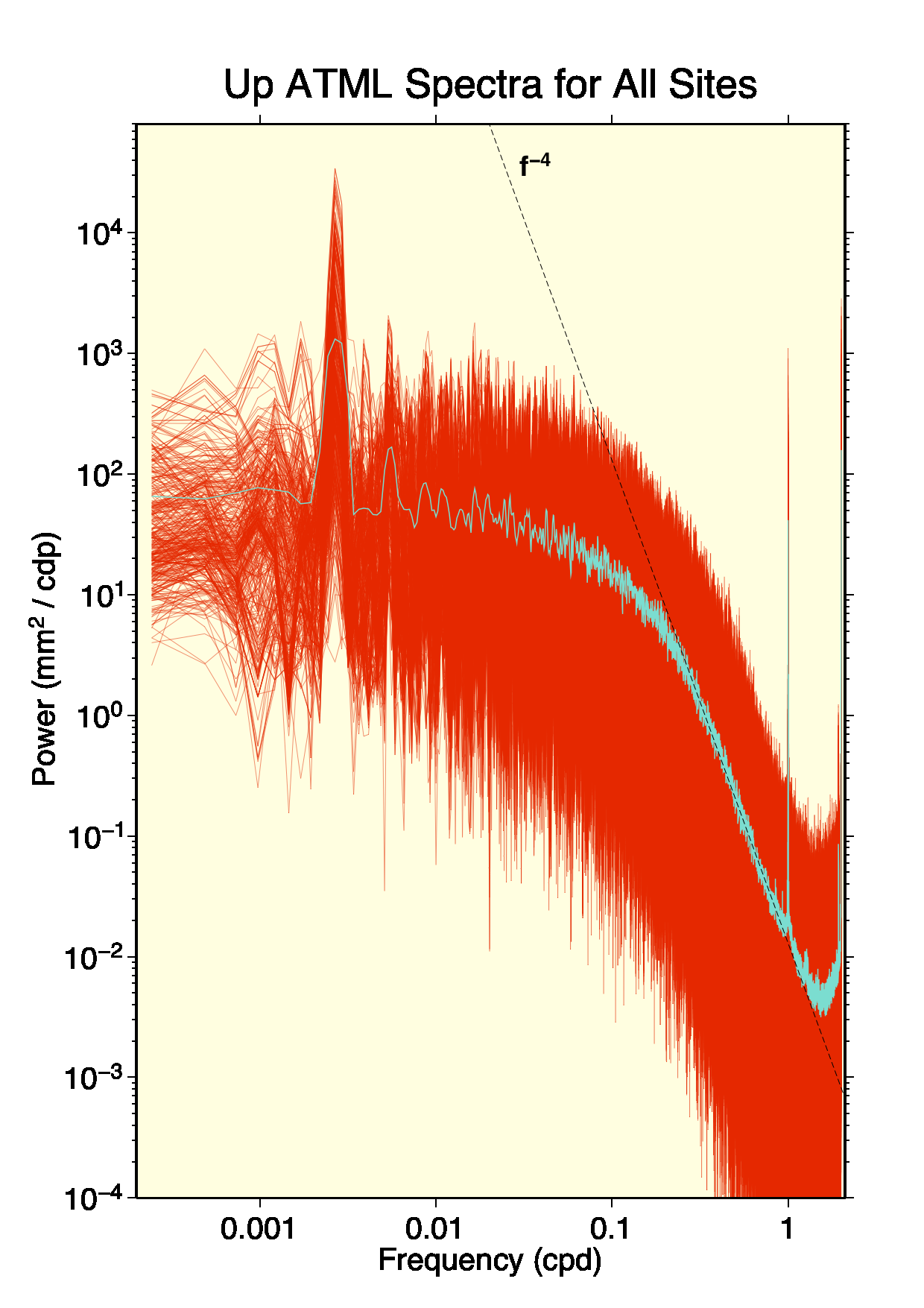
- the stacked mean PSD for this ensemble of stations is shown by the turquoise line, which follows a power-law with spectral index of -4 for frequencies >0.4 cpd (ignoring the strong S1 & S2 tidal lines; the S2 line is broadened by being at the Nyquist sampling limit)
- the fit for the mean atmosphere pressure loading trend from 0.4 cpd upward (but omitting the tidal bands around 1.0 & from 1.13 cpd onward) is approximately:
PSDUp = 0.013 mm2/cpd * f -4indicated by the dotted line in the plot above - integrating this power law from 1/1 cpd to infinity & from 1/7 cpd to infinity, assuming the same -4 power law extends to the highest possible frequencies, gives these variances, respectively:
Var (1/1 -> inf)Up = 0.00433 mm2Var (1/7 -> inf)Up = 1.486 mm2or equivalently these scatters, respectively:
RMS (1/1 -> inf)Up = 0.066 mmRMS (1/7 -> inf)Up = 1.219 mm - for a GPS dUp measurement with a basement error of about 2.2 mm for weekly observations (as found from the IGS repro1 results), one must expect daily measurements to have errors no smaller than sqrt(7) times larger if there are no temporal error correlations (higher otherwise) or about 5.8 mm; so the actual atmospheric pressure dUp loading variations are much smaller than the GPS detection limit for 1 d intervals (by about two orders of magnitude on average) but the average load variations are within a factor of ~2 of the GPS WRMS noise floor for weekly dUp integrations & can even exceed the GPS noise floor at some extreme stations (considering the spatial variation in PSD spans about a factor of 10 upward and downward, or equivalently a factor of 3 to 4 in RMS)
- consequently, this suggests that there is some loss, on average, in GPS sensitivity to atmosphere loading with the present IGS weekly integrations when load corrections are not applied, but this would not be the case with daily frame integrations
- tidal EOP variations
- most current models & recommendations should already be implemented
- this includes the subdaily polar motion libration terms introduced in 2005 & previously called “high-frequency nutation”, which can be computed using fortran routines PMsdnut.f or PMSDNUT2.f
- key exception is the addition of UT1 libration effects, introduced in late 2009
- see IERS Conventions (2010) Table 5.1b for coefficients of 11 largest semidiurnal UT1 libration terms or use the new fortran routine UTLIBR.F from A. Brzezinski
- note that the maximum UT1 libration effect is 105 µas (peak-to-peak) or 13 mm at GPS altitude, which probably aliases strongly into the orbit parameters
- standard IGS Earth rotation parameterization should be used, with daily (noon) estimates for the x,y coordinates of polar motion, their time derivatives over the 24 hr surrounding each noon, & (nominal) length-of-day (LOD) variations over the 24 hr surrounding each noon
- each set of daily ERPs should be determined freely, without any a priori or continuity constraints
- tropospheric propagation delays
- for details, refer to IERS Conventions (2010) section 9.2
- a priori meteorological data sources:
- [1] local sensor met files (which however are only available for a few sites), or
- [2] the fortran routine GPT2.f returns location- & season-dependent values for local pressure, temperature, temperature lapse rate, water vapor pressure, hydrostatic and wet mapping function coefficients ah & aw, and geoid undulation based on a 5 x 5 degree gridded fit to a long history of ECMWF fields; this updated version gives much better spatial and temporal resolution than the prior GPT.f model available at the IERS Conventions website; please refer to the README comments for further information; the associated external grid file is available here & should be placed in the directory where the routine is run or else the subroutine open call modified
- [3] retrieved from a numerical weather model, as for the ECMWF global values provided by the service at the Technical University of Vienna in the form of gridded hydrostatic zenith delays
- a priori hydrostatic delays in the zenith direction should be computed from the surface pressure from any of the sources above according to the formula of Saastamoinen (1972) as given by Davis et al. (1985) & shown as eqn (9.11) in IERS Conventions (2010) Chapter 9
- a fortran routine for this computation is available at DRYSAAS.f
- or retrieved directly in this form based on a numerical weather model, as for the gridded ECMWF values provided by the service at the Technical University of Vienna
- a priori wet delays in the zenith direction can also be computed provided that the local temperature and water vapor pressure are known (see above):
- using the sum of the a priori hydrostatic and wet zenith delays will ensure that the tropospheric parameter adjustments that are more nearly zero-mean
- a test at NGS using a week of data from about 235 globally distributed stations found that using GPT2 for a priori meteo values improved the residual zenith tropo delay adjustments from 42 +/- 64 mm (assuming a relative humidity of 0.50 everywhere) to 3 +/- 54 mm
- a priori azimuthally symmetric line-of-sight delays should be computed using either:
- [1] the location- & season-dependent VMF1_HT.F mapping function model; this requires input values for the hydrostatic and wet mapping function coefficients ah & aw, which can be passed from the GPT2.f routine described above; continued use of the GMF mapping function is no longer recommended
- [2] or a mapping function based on retrieval coefficients from a numerical weather model, as for the ECMWF global values provided by the
service at the Technical University of Vienna for the VMF1 mapping function model
- a priori asymmetric line-of-sight delays caused by the mean troposphere distribution (represented by a spherical harmonic expansion to degree and order 9) can be evaluated using the fortran routine APG
- note that the north & east gradients from this routine should be used with the gradient model by G. Chen & T.A. Herring (“Effects of atmospheric azimuthal asymmetry on the analysis of space geodetic data”, J. Geophys. Res., 102(B9), 20,489-20,502, doi: 10.1029/97JB01739, 1997), also described in APG
- note also that test results using the APG model have not verified its usefulness, so it is not recommended for general adoption at this time
- note that using the simpler GPT2 routine (with VMF1_HT) rather than more realistic a prioris derived from in situ data or numerical weather models can partially compensate for sub-seasonal atmospheric pressure loading effects at a level probably smaller than ~1 mm in annual height variation (see J. Kouba, 2009 & P. Steigenberger et al., 2009); this effect arises due to systematic limitations of the GPT2 model that fail to capture the full measure of spatial and temporal variations of the troposphere (together with small differences in the dry & wet mapping functions, which are very sharp functions of elevation cutoff angle); consequently, the magnitude of this compensation effect is a strong function of the AC elevation cutoff angle; in this respect note also that the Steigenberger et al. analysis included GPS data with elevation angles down to 3 degree (with elevation-dependent weighting); ACs with higher elevation cutoff angles will experience smaller loading compensation
- but note further that ray-tracing of direct a priori slant delays using spatially & temporally high-resolution troposphere models should be superior, in principle, but sufficient global models are not yet available; however, it has not been found so far that residual troposphere parameters can be eliminated from space geodetic solutions, a step that would bring significant precision improvements if the slant delays can be determined accurately enough
- residual tropospheric delays should be parameterized in the GNSS data analysis on the assumption that they are predominantly due to unmodeled variations in the wet component of the troposphere zenith delay (that is, using wet mapping function partials) as well as unmodeled azimuthal gradients
- GNSS data are sensitive to zenith delay changes over intervals as short as the observation sampling, but parameterization at hourly intervals is much more efficient & usually satisfactory
- a minimal gradient parameterization involves one N-S & one E-W parameter at the beginning & end of each day of data for each station, with continuous linear variation during the day
- the Chen-Herring (1997) gradient mapping function is recommended; see updated IERS Conventions (2010) section 9.2:
mg(e) = 1 / [sin(e)tan(e) + 0.0031] - where “e” is the observation elevation angle. Unlike other gradient mapping functions, this one is not affected by a singularity at very low elevations & should also be used with the APG a priori gradient model.
- for gradient estimation, an elevation cutoff angle no higher than 10 degrees is recommended; otherwise station height accuracies will suffer
- a priori parameter constraints are not needed & are strongly discouraged
- higher-order ionospheric corrections
- for details, refer to IERS Conventions (2010) section 9.4
- a software package has been developed by M. Hernandez Pajares & colleagues to compute the 2nd order ionosphere correction; it is available at this site
- the software is entirely new, with contributions & debugging from an informal working group of volunteers
- only the 2nd order correction, which is larger & for which there is a clear consensus on how it should be applied, is included currently; additional higher-order terms can be incorporated in the future
- analysis constraints
- a limitation in IGS operational & repro1 products is the application of unremovable constraints by some ACs (see R. Ferland, 2010)
- unremovable continuity constraints, for example, can act as biased filters & cause significant signal distortions (see J. Ray, 2008)
- these can be particularly insidious when applied to pre-reduced parameters, such as orbit estimates, & are especially difficult to justify for GNSS processing where almost every parameter is highly observable
- consequently, some AC contributions are routinely excluded from IGS product combinations
- for repro2, ACs are asked to avoid any solution over-constraints, applying pre-removed or unremovable constraints no tighter than noise levels & ensuring that any other constraints are strictly removable — see reprocessing recommendations on p. 10 of the IGS 2010 Workshop in Newcastle
- failure to meet this condition may force full AC exclusion from the product combinations
- self-certification
- each AC will be asked to certify its compliance with these standards, noting specific areas of deviation
- all AC metadata errors reported in the weekly SINEX combination reports should be corrected
- all ACs should also ensure that their analysis processing summary files at the IGS Central Bureau are up to date
Repro2 preliminary product combinations for evaluation:
- The IGS contribution to ITRF2013 – Preliminary results from the IGS repro2 SINEX combinations (2014) by P. Rebischung et al., a presentation at the Fall 2014 American Geophysical Union Meeting
- Preliminary Analysis of IGS 2nd Reprocessed Orbits by K. Choi, a poster presentation at the 2015 European Geosciences Union
Repro2 TRF combinations:
- Combination of the IGS repro2 Terrestrial Frames by P. Rebischung et al., a poster presentation at the 2015 European Geosciences Union
- The IGS Contribution to ITRF2014 (2015) by P. Rebischung, B. Garayt, Z. Altamimi, X. Collilieux, a presentation at the 26th IUGG General Assembly, Prague, 28 June 2015
- Combined orbits and clocks from IGS second reprocessing by J. Griffiths, an article in the Journal of Geodesy
3rd Data Reprocessing Campaign (REPRO3)
Objective
By the start October 2019, the Analysis Centers (ACs) of the International GNSS Service will begin the third reanalysis of the full history of GPS data collected by the IGS global network since 1994 in a fully consistent way using the latest models and methodology.
Reference Frame
The final version of the repro3 reference frame SINEX file is now available at:
- ftp://igs-rf.ign.fr/pub/IGSR3/IGSR3_2077.snx
- ftp://igs-rf.ign.fr/pub/IGSR3/IGSR3_2077.ssc (without covariance matrix)
The associated discontinuity list and post-seismic deformation models are respectively available at:
Stations categorized by priority for Reference Frame Determination for repro3, provided by Paul Rebischung
Antenna Modelling
The ANTEX file to be used for repro3 can be downloaded from igsR3_2077.atx
The antenna model was selected based on tests of different ANTEX files and assessing their impacts upon the reference frame for the period starting in 2017 through to the end of 2018
Test Reprocessing results from Paul Rebischung, with solutions provided by CODE, ESA, GFZ, GRG, and TuGraz
IERS Conventions (2010)
- should be implemented
- please also check for any ongoing electronic updates
Mean Pole tide
As of early 2018, the IERS officially adopted a new (linear) mean pole for purposes of computing rotational deformation (pole tide). See the updated Chapter 7 at http://iers-conventions.obspm.fr/chapter7.php
By adopting a linear mean pole, no corrections are required to C21/S21 going forward.
- only to be implemented during the reprocessing run. Do not implement this in the operational stream otherwise a discontinuity in the velocities will be introduced
- There is the possibility of applying this correction at the solution level, rather than at the observation level
- Here is a presentation by John Ries outlining the case for a linear mean pole model here
Sub-daily EOP model
HF-EOP recommends the use of the Desai&Sibois/Egbert model for diurnal and sub-diurnal EOP variation. Coefficients for this model and software to generate EOP predictions can be obtained from https://ivscc.gsfc.nasa.gov/hfeop_wg/
Solar radiation pressure models
The SRP model to be applied is dependent upon the constellation, and satellite block being processed.
- ACs should upgrade from just ECOM1 modelling, with the exception of GPS Block IIF and IIR satellites
- ECOM2 or JPL GSPM modelling should be used for other GPS Block Types, or a box-wing model
Earth albedo models
Reflected (albedo) and retransmitted radiation from the Earth may cause scale (1 – 2 cm) and translational effects at GNSS altitudes; see:
A recommended model for these effects,in the form of Fortran source code was originally developed within the scope of the IGS Orbit Modeling Working Group for repro2, this has recently been updated by Thomas Herring to include new values for GLONASS-M and GLONASS-K satellites (31 July 2019).
- ERPFBOXW.f Computation of Earth Radiation Pressure acting on a box-wing satellite
- SURFBOXW.f Computes the force on the satellite surfaces for a given radiation vector
- PROPBOXW.f Provides the satellite dimensions and optical properties for different satellites blocks:
- GPS: GPS-I,GPS-II,GPS-IIA,GPS-IIR,GPS-IIR-A,GPS-IIR-B,GPS-IIR-M,GPS-IIF,GPS-IIIA
- GLONASS: GLONASS-M,GLONASS-K
- GALILEO: IOV, FOC
Ocean Tide Model
FES has recently been updated to FES2014b, a description of the products can be found here. A link to the spherical harmonic coefficients in geopotential be found at the bottom of the page.
Satellite Transmit Power (Antenna Thrust)
Technical note on satellite transmit power for GPS and GLONASS, by Peter Steigneberger is available from here.
Third body effects
- recommend ACs apply all planets into model
Time variable gravity
Other ITRF observing techniques are considering the highest fidelity time-variable gravity model, this is not strictly required for GNSS orbits, but it will be important to stay consistent with their implementation.
Loading Models
- should be consistent with the TVG model, and again consistent across all observing techniques
- Long Product Name Convention
Data Products
use RINEX3 in preference to RINEX2 Provide solutions in updated SINEX formats that support RINEX3
Last Updated on 18 May 2026 16:56 UTC